Intro to Partisanship Modeling

In the Persuasion Analytics and Targeting (review available here) class, the first predictive modeling assignment was to use both a regression based classifier and a tree based classifier to create four predictive models, two voter turnout models and two partisanship models. I will walk through the process I used to create a partisanship model using logistic regression. For this exercise, we acted as if we were building models for a candidate in the 2016 election. For the first project, I used the default settings (I worked on parameter tuning in later weeks). In this post I will look at creating a pipeline for data preparation and parameter tuning.

Using logistic regression was a great way to practice using a tried and true machine learning technique. It is well studied and almost every program and framework has an optimized process for running it. In this tutorial, I use sci-kit learn to implement a logistic regression model to predict voter partisanship.

The Data

The data set was provided for the class and is actual campaign data used to create predictive models. It contains a combination of voter file data (publicly available), demographic information from the Census, commercially purchased enhancements, and derived fields (number of poeple in household, number of last 3 elections voted in, etc.). The data also contained ID responses from voter ID calls since this is actual (anonymized) campaign data. I cannot share it or show too much of the data exploration, but I can walk through the process for building models.

The sample data was from a state with party registration, so we had nearly complete coverage for which party affiliation. Some may be asking why we would create a partisanship model in this case. There are always new voters that may not have yet registered with a party or registered Independent/3rd-party who share a lot of similarities with voters in one party. In my experience, a lot of voters may claim to be Independent or "just vote for the person, not party," but have exclusively voted for one party their entire adult lives. Creating a partisanship model will help more helpfully assign them to a party for targeting purposes. Additionally, it can be helpful to try modeling exactly how partisan a voter happens to be. There is no "partisanship requirement" to party registration.

Due to the commercial nature of the data, I will not share the data exploration code/results. However, it was quickly clear that several columns were correlated with each other. This multicollinearity will throw off logistic regression, I either had to manually pick between the columns or use regularization. I decided to test both L1 and L2 regularization rather than manually pick columns. More on that below.

Data Preparation

The first step was to set up my environment (Python 3 in a Jupyter notebook) and import the necessary libararies.

import pandas as pd
import numpy as np

from sklearn.preprocessing import StandardScaler
from sklearn.linear_model import LogisticRegression
from sklearn.pipeline import Pipeline
from sklearn.metrics import classification_report 
from sklearn.metrics import roc_auc_score
from sklearn.metrics import auc
from sklearn.metrics import roc_curve
from sklearn.grid_search import GridSearchCV

import matplotlib.pyplot as plt

The next step was to remove columns that were derived from the party registration information on the data file. Namely, the number of registered Democrats/Republicans in the household, and percent Democrats/Republicans in the household household. ::python data = pd.read_csv('./data/FX_indicators.csv', index_col='VOTER_ID') data.head()

to_remove = ['colums', 'to', 'remove']

data1 = data.drop(to_drop, axis = 1)

In checking the file, several columns had categorical data and flags ('Y' or 'N'), which needed to be recoded to binary variables.

data1['sample_column'].replace({'N': 0, 'Y':1}, inplace=True)

The data from class had a random number (1-3) to be used for dividing the data between training and test sets. 1 and 2 were for training and 3 was a test set. In a real world setting, I would have had to separate out the train and test sets manually.

train = data1[data1['SET_NO']!=3]
train.drop('SET_NO', axis=1, inplace=True)

test = data1[data1['SET_NO']==3]
test.drop('SET_NO', axis=1, inplace=True)

Once the data was ready, I separated out the target variable (party) so that it could be fed into the model.

target = 'target_column'

y_train = train[[target]]
X_train = train.drop(target, axis = 1)

y_test = test[[target]]
X_test = test.drop(target, axis = 1)

Modeling

As mentioned earlier, this data contained a lot of correlated fields which is problematic for logistic regression so I tested two methods of regularization. Additionally, I used the scikit-learn standard scaler to normalize all of the columns. This was all loaded into a pipeline along with different values for C to test how strong of regularization to use.

logistic_pipeline = Pipeline([('scl', StandardScaler()),
                        ('clf', LogisticRegression())])

Next, I set the parameters I want to search. The model tested five values for both L1 and L2 regularization.

param_grid = [{'clf__penalty':["l1","l2"],
           'clf__random_state': [45],
           'clf__C':[0.001, 0.01, 0.1, 0.5, 1],
          }]

With the pipeline ready, I used 5 fold cross validation (link) to compare the model parameters. Ultimately the model will be used to give a probability score to everyone rather than just labels. Given this goal, I used AUC to compare the models (and pick the best).

gs2=GridSearchCV(estimator=logistic_pipeline,
           param_grid=param_grid,
           scoring='roc_auc',
           cv=5,
           n_jobs=-1)

And finally, the code below starts the model fitting process.

gs2=gs2.fit(X_train, y_train.values.ravel())
print(gs2.best_score_)
print(gs2.best_params_)

The best model was Logistic regression with L2 regularization and C=1 which got an average AUC of .78 on the training data.

I then ran this final model on the test set and plot the ROC curve.

y_trained = gs2.predict_proba(X_test)[:, 1]

false_positive_rate, true_positive_rate, thresholds = roc_curve(y_test, y_trained)
roc_auc = auc(false_positive_rate, true_positive_rate)

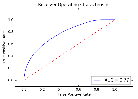
The AUC was a respectable .77 on the test data. This leaves us with a pretty good model. Even with a good score it is important to check some model diagnostics.

Diagnostics

Rather than just view the AUC metric, I will plot the ROC curve to see how the model performs at different thresholds and versus random guessing (the red line in the plot)

plt.title('Receiver Operating Characteristic')
plt.plot(false_positive_rate, true_positive_rate, 'b',
label='AUC = %0.2f'% roc_auc)
plt.legend(loc='lower right')
    plt.plot([0,1],[0,1],'r--')
plt.xlim([-0.1,1.2])
plt.ylim([-0.1,1.2])
plt.ylabel('True Positive Rate')
plt.xlabel('False Positive Rate')
plt.show()
plt.savefig('aucplot.png')

Next, I will plot the learning curves for the final model. The package mlxtend is fantastic and contains a lot of useful functions including a convenience function for plotting a confusion matrix. The catch is that is only takes in labels. While this will not be the ultimate use of the model, I will use the following code to predict labels over the test set and then plot a confusion matrix.

from mlxtend.plotting import plot_confusion_matrix
from sklearn.metrics import confusion_matrix
y_trained2 = gs2.predict(X_test)
conf_m = confusion_matrix(y_test.values.ravel(), y_trained2)

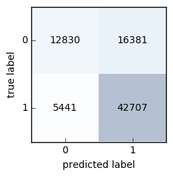
This plot shows the model is great at successfully flagging democrats but struggles to identify Republicans. It is overly optimistic about flagging them as a 1 (democrat). Another view is below.

cl_report = classification_report(y_test.values.ravel(), y_trained2)
print(cl_report)

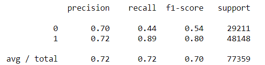
Even though we will use the model to create scores, it is good to know that it can be optimistic in its class assignments. If we were to use the model to assign categories (Dem/Repub), it would be worth exploring changes to the threshold used to assign labels. Click here more information about the confusion matrix and associated metrics.

Since this ended up being a pretty good predictive model, I will use the following code to save the pipeline for later use.

filename = 'l2logisticPartisanshipFull.sav'
dump(gs2, open(filename, 'wb'))

With the model complete, the final step would be to score it against the voter file. With a good partisanship model created, I will turn my attention to candidate support and voter turnout models in future posts.