Building Candidate Support Models with Ensembles - The Frankenstein Method

Having a model to predict a voters likelihood to support your candidate is the backbone of a campaign's data operation. Combined with voter turnout models, you can more effectively plan your strategy, allocate resources, and contact the right voters at the right time. There is a fine art to building these models but instead of focusing on that, I will walk through one strategy of cobbling together several simpler models. Basically it's the kitchen sink or Frankenstein's monster approach to machine learning. Unlike in the preivous post, there will not be any parameter tuning; I will instead use the defaut paratmeters of all of the models. Then I will then walk through a few methods of how to combine them into a well rounded model to predict which voters are likely to support your candidate.

Getting the IDs

I am using the same data as before, industry grade voter file with commercial enhancements that has actual candidate IDs appended. In a regular campaign, there would be a lot of effort needed to call voters (either with volunteers or vendors) to ask who they are supporting. Once we have enough IDs for the candidates in our election, we can use them to build a model to predict how the rest of the voters are likely to feel. This is not an exact science however. I know that using data and models in elections is out of favor right now in the press, but a well made (and more importantly well applied) model is still essential to a campaign. While they cannot be the only consideration in campaign strategy, they can give a great insight into which groups of voters need more outreach, and how best to engage them.

Traditionally, campaigns will use a 5 point scale for identifying support 1-Strong Supporter, 2-Lean Supporters, 3-Undecided, 4-Lean Opponent, 5-Strong Opponent. When building the model you will need to decide what it is you are modeling. In our case, this is who is a 1 or a 2 versus all of the rest. For these models a score of 100 is as confident as we can be that the voter in question is a supporter, while a 0 is a very confident estimate they really do not support our candidate. NOTE - a middle score does not mean that the voter is undecided! It means the model is undecided on whether they are likely to be a supporter, not that the voter is undecided. Unless the model is specifically built to find undecided voters, do not make this mistake. This is a common mistake made by a lot of experienced professionals. While mid-scoring voters is still a potentially useful group to call for IDs, it does not mean they are undecided or persuadable. You can specifically model whether they are undecided but cannot assume that is part of all candidate models.

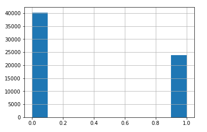
As I mentioned, I will use both 1s and 2s as supporters for this model. In this case decision is arbirtrary, but you should decide what makes the most sense in a specific race. As in the last post, I will remove columns that are derived or informed by the results of the ID so we do not use data from IDs we have not done yet. Below is code to look at the counts of each ID and produce a histogram.

%matplotlib inline
data[target].hist()
data['CAND1_LD2'].value_counts()

The next step is to split the data into a training set and a test set. The test_size parameter takes a percentage of observations to move to a test set and automatically shuffles and splits. In this case we will keep 1/3 of the data for a test set.

data1 = np.array(data.drop(target, axis=1))
Y = np.array(data[target]).astype(np.integer)
X=data1

test_size = 0.33
seed = 55
X_train, X_test, Y_train, Y_test = train_test_split(X, Y, test_size=test_size, random_state=seed)

Since many classifiers are sensitive to outliers and larger numeric values (such as logistic regression), I run everything through the scikit learn standard scaler. In the previous post I had put this step in a pipeline. This time I am using it separately since I am creating several separate models.

ssc = StandardScaler()

X_train1 = ssc.fit_transform(X_train)
X_test1 = ssc.fit_transform(X_test)

Since the data is imbalanced, using stratified k fold will balance the data used during cross validation to give a more helpful measure of the accuracy. By balancing the classes, the model will be tested equally on both 1's and 0's and eliminates the risk that a test will have just one class in it.

from sklearn.model_selection import StratifiedKFold
cv1 = StratifiedKFold(n_splits=5)

Next, I create a list of three models (Naive Bayes, Random Forest, and Linear Discriminant Analysis) with no parameter tuning to blend together later. Each is appended with a label for use later. I also set the class weight parameter to balanced, when available, to help offset the class imbalance.

estimators1 = []

model1 = GaussianNB() 
estimators1.append(('nb', model1))

model2 = RandomForestClassifier(class_weight = 'balanced') 
estimators1.append(('rf', model2))

model3 = LinearDiscriminantAnalysis()
estimators1.append(('lda', model3))

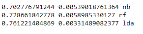
The first method of blending is to have each model vote on which class (supporter or not) to assign each voter. The code also prints out the accuracy of each individual model and the accuracy for blended model. (Link for more info)

from sklearn.ensemble import VotingClassifier

for i in estimators1:
scores = model_selection.cross_val_score(i[1], X_train1, Y_train, cv=cv1, scoring='accuracy')
print(scores.mean(), scores.std(), i[0])

ensembles = VotingClassifier(estimators1) 
results = model_selection.cross_val_score(ensembles, X_train1, Y_train, cv=cv1)

print(results.mean(), results.std())

As I hoped, the voting model is more accurate overall than each of the models individually. I, for whatever really nerdy reason, find this a fascinating part of machine learning. Each model balances out flaws in the other models to create a more accurate prediction. Below, I create a plot that shows how many people were assigned each label versus what the test data said their label was. Correct answers have the same label (so boxes 0,0 and 1,1). Each cell is shaded based on how many observations fall into each category. There is a chart for each indidvidual model and then the voting ensemble.

from mlxtend.plotting import plot_confusion_matrix
from sklearn.metrics import confusion_matrix

gs = gridspec.GridSpec(2, 2)

fig = plt.figure(figsize=(10,8))

for clf, lab, grd in zip([model1, model2, model3, ensembles], 
                     ['NB', 
                      'Random Forest', 
                      'LDA',
                      'Ensemble'
                      ],
                      itertools.product([0, 1], repeat=2)):

    clf.fit(X_train, Y_train)
    y2 = clf.predict(X_test)

    x = confusion_matrix(Y_test, y2)
    #ax = plt.subplot(gs[grd[0], grd[1]])
    plot_confusion_matrix(conf_mat=x, )
    plt.title(lab)
plt.show()

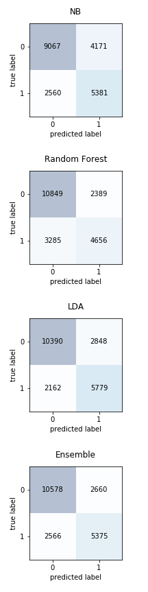
In the first chart you can see the Naive Bayes classifier is doing well overall while the Random Forest is very accurately classifying the 0's but struggling with the 1's. The LDA model does a surprisingly good job with the highest accuracy but the blended model balance between precision and recall. Basically, it predicts both classes better than each of the individual models.

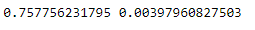
Next is a stacking model where a meta-model is fit on top of the results from other models. Mlxtend has two useful functions for creating this model, StackingClassifier and StackingCVClassifier. The second is shown below.

from mlxtend.classifier import StackingCVClassifier

m1 = GaussianNB()
m2 = RandomForestClassifier(class_weight = 'balanced')
m3 = LinearDiscriminantAnalysis()

lr = LogisticRegression(class_weight = 'balanced')

sclf2 = StackingCVClassifier(classifiers=[m1, m2, m3], 
                      meta_classifier=lr, 
                        use_probas = True, cv=cv1)

scores = model_selection.cross_val_score(sclf2, X_train1, Y_train, cv=cv1, scoring='accuracy')
print(scores.mean(), scores.std())

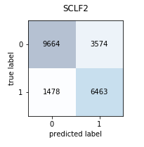
The code above fits the same three models from before and then uses their predictions as input for the final logistic regression model. The function also takes care of splitting the training data between the three models and the final meta-model as well as the splits needed for cross-validation. These are all fit using the same cross-validation setup as before so that comparing performance is easier. Below is a confusion matrix to evaluate the performance.

As with the Voting Classifier, this model has great balance in predicting both classes accurately. It does slightly better than the voting ensemble, but both are surprisingly accurate.

The StackingClassifier model has additional options worth exploring whether to include the "use_proba" which uses probability estimates from the base models as input. Also, you can tune parameters (using cross-validation) on the input models and/or the meta model. But those are topics for a future post, but you can learn more here in the meantime.

Using the methods outlined above, you can quickly evaluate the performance of several models (possibly for use later) as well as blend together their predictions . This is a common step in a manchine learning workflow and can be used in a variety of predictive modeling tasks.